Page 3 - Computers and Technology for Science

03-SC-Spreadsheet 5/30/07 3:32 PM Page 89

Learning Computers and Technology for Science | Spreadsheets | Activity 1

PROCEDURES

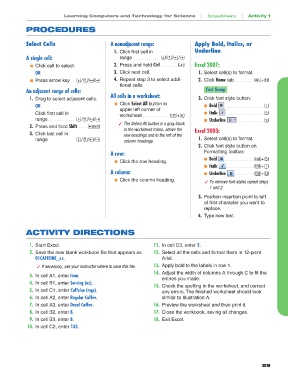
Select Cells A nonadjacent range: Apply Bold, Italics, or
1. Click first cell in Underline
A single cell: range . . . . . . . . . . . . . . . . . . . . . . . . . . ˘/¯/≤/≥

! Click cell to select. 2. Press and hold Ctrl . . . . . . . . . . . . . . . . Ç Excel 2007:
OR 3. Click next cell. 1. Select cell(s) to format.

! Press arrow key. . . . . . ˘/¯/≤/≥ 4. Repeat step 3 to select addi- 2. Click Home tab . . . . . . . . . . . . . . . . . . å+H
tional cells.
An adjacent range of cells: Font Group
1. Drag to select adjacent cells. All cells in a worksheet: 3. Click font style button:
OR ! Click Select All button in ! Bold . . . . . . . . . . . . . . . . . . . . . . . . . . . . . . . . . . . . 1
upper left corner of
Click first cell in worksheet. . . . . . . . . . . . . . . . . . . . . . . . . . Ç+A ! Italic . . . . . . . . . . . . . . . . . . . . . . . . . . . . . . . . . . . 2
range . . . . . . . . . . . . . . . . . . . . . . . . . . ˘/¯/≤/≥ ! Underline . . . . . . . . . . . . . . . . . . . . . . . . . 3
" The Select All button is a gray block
2. Press and hold Shift. . . . . . . . . . Í in the worksheet frame, above the Excel 2003:
3. Click last cell in row headings and to the left of the
range . . . . . . . . . . . . . . . . . . . . . . . . . . ˘/¯/≤/≥ column headings. 1. Select cell(s) to format.
2. Click font style button on
A row: Formatting toolbar:
! Click the row heading. ! Bold . . . . . . . . . . . . . . . . . . . . . . . . . . . Ç+B
! Italic . . . . . . . . . . . . . . . . . . . . . . . . . . Ç+I
A column: ! Underline . . . . . . . . . . . . . . . . . . Ç+U
! Click the column heading. " To remove font styles repeat steps
1 and 2.
3. Position insertion point to left
of first character you want to
replace.
4. Type new text.

ACTIVITY DIRECTIONS

1. Start Excel. 11. In cell C3, enter 5.
2. Save the new blank workbook file that appears as 12. Select all the cells and format them in 12-point
01CAFFEINE_xx. Arial.
" If necessary, ask your instructor where to save this file. 13. Apply bold to the labels in row 1.
14. Adjust the width of columns A through C to fit the
3. In cell A1, enter Item.
entries you made.
4. In cell B1, enter Serving (oz).
15. Check the spelling in the worksheet, and correct
5. In cell C1, enter Caffeine (mgs). any errors. The finished worksheet should look
6. In cell A2, enter Regular Coffee. similar to Illustration A.
7. In cell A3, enter Decaf Coffee. 16. Preview the worksheet and then print it.
8. In cell B2, enter 8. 17. Close the workbook, saving all changes.
9. In cell B3, enter 8. 18. Exit Excel.
10. In cell C2, enter 135.

89